Complexity Theory, Relativity and The Theory of Everything

This week’s guest post is by Matthew Butler, who shows us some insights about how the relationship between complexity and performance can be less than obvious in multiple ways. Matthew is a systems architect and software engineer developing systems for physics research, network security, law enforcement and the Department of Defense. He primarily works in C/C++ and Modern C++ and can be found on Twitter.

There’s a story that’s been told for years about Jon Bentley (Programming Pearls, Addison-Wesley, 1986) coming excitedly into Bjarne Stroustrup’s office one day and posing a problem to him:

“Insert a sequence of random integers into a sorted sequence, then remove those elements one by one as determined by a random sequence of positions. Do you use a vector or a linked list?”

I’m not sure if this is a true story or even if it even happened that way, but it brings up an interesting point about algorithm complexity and data structures.

If we analyze the problem from a strict complexity viewpoint, linked lists should easily beat arrays. Randomly inserting into a linked list is O(1) for the insertion and O(n) for finding the correct location. Randomly inserting into an array is O(n) for the insertion and O(n) for finding the correct location. Removal is similar.

This is mainly because arrays require the movement of large blocks of memory on insertion or deletion while linked lists just swizzle a few pointers. So, by a strict complexity analysis, a list implementation should easily win.

But does it?

I tested this hypothesis on std::list, which is a doubly-linked list, and std::vector. I did this for a data set of a small numbers of elements: 100, 1,000, 2,000, 3,000, 4,000, 5,000, 6,000, 7,000, 8,000, 9,000 & 10,000. Each run was timed using a high-resolution timer.

Code segment for std::list:

while (count < n)
{
    rand_num = rand();

    for (it = ll.begin(); it != ll.end(); ++it)
        if (rand_num < *it)
            break; 
    ll.insert(it, rand_num);

    ++count;
} 

while (count > 0)
{
    rand_num = rand() % count;

    it = ll.begin();
    advance(it, rand_num);
    ll.erase(it);

    --count;
}

Code for std::vector:

while (count < n)
{
    rand_num = rand();
    for (i = 0; i < count; ++i)
        if (rand_num < vec[i])
            break;
    vec.insert(vec.begin() + i, rand_num);
    ++count;
}

while (count > 0)
{
    rand_num = rand() % count;
    vec.erase(vec.begin() + rand_num);

    --count;
}

Code for an optimized std::vector that uses a binary search to find the insertion point and reserve() to keep the vector from being relocated as it grows.

vec.reserve(n);

while (count < n)
{
    rand_num = rand();
    it = std::lower_bound(vec.begin(), vec.end(), rand_num);
    vec.insert(it, rand_num);
    ++count;
}

while (count > 0)
{
    rand_num = rand() % count;
    vec.erase(vec.begin() + rand_num);

    --count;
}

 

The Results

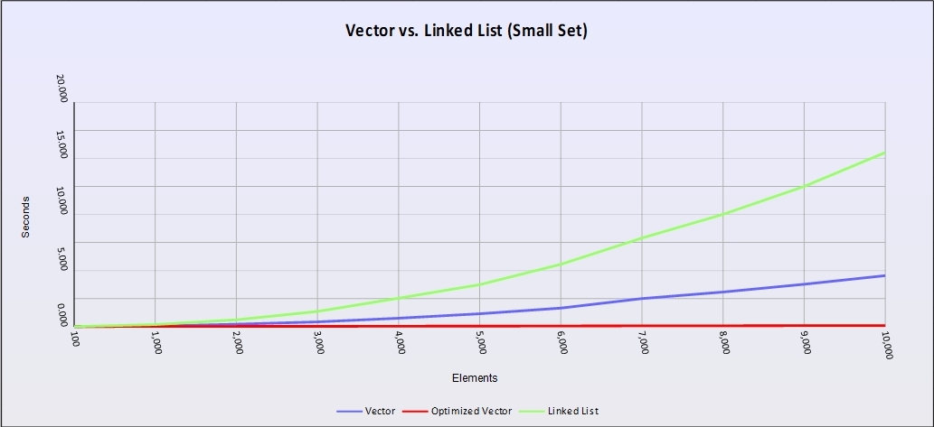
Figure 1 – Performance curves (load vs time) for std::list (green), std::vector (blue) and an optimized std::vector (red) using integers. A lower line means better performance.

 

Clearly, std::list loses badly. But the surprising result is the nearly flat-lined performance of the optimized version of std::vector. So how did we get graphs that defy what complexity analysis told us we should see?

This is one of the central failings of complexity analysis. Complexity analysis only looks at the data structure & algorithm as if they’re running in the aether. It doesn’t take into account the relativistic effects of the hardware we’re running on. In this case, the CPU cache and pre-fetcher work under the hood to make sure that the data we need is pre-loaded into the cache lines for faster access.

std::vector, which is just a block of memory, is easy for the pre-fetcher to reason about given our linear access patterns. It anticipates the next blocks of memory we’ll want to access and has them loaded and ready when we try to access them.

Linked lists, on the other hand, can’t be pre-fetched since each new link points somewhere else in memory and the pre-fetcher can’t reason about that. Each move down the list becomes a cache miss causing the CPU to spill the cache line and re-fill it with a different block of memory.

This means that accessing the next element goes from 0.9ns (if it’s in the cache already) to 120ns to get it loaded from main memory. In this case, the best quality of std::list – the ability to swizzle some pointers to insert or delete – is also it’s Achilles heal on cache-based architectures.

If you looked at the code above, you also noticed that I used random access to delete from the vector. While this may seem to be an advantage, it’s really not. There’s no guarantee that the next value to be removed is anywhere near the last one and the pre-fetcher has no understanding of how you structured your data in memory. It just sees memory as one long, formless stream. That means that you potentially take cache misses depending on how big the array is and where you’re looking.

But what about the use of binary search?

That’s a pseudo-random access pattern which should cause a fair amount of cache misses. And yet the “performance-tuned” std::vector was blazingly fast even with it’s cache misses.

There are a few things to keep in mind:

• We did O(log n) accesses for a binary search which is far fewer than a linear traversal which is O(n).

• The branch predictor works to make the single if() statement inside the binary search more efficient by predicting which outcome is more likely on each loop.

• We pre-allocated the entire array which means that it didn’t have to be relocated as it grew and potentially ran out of space.

Larger Data

But what happens if the data we’re handling isn’t an integer? What if it’s something larger, like a 4K buffer?

Here are the results using the same code but using a 4K buffer.

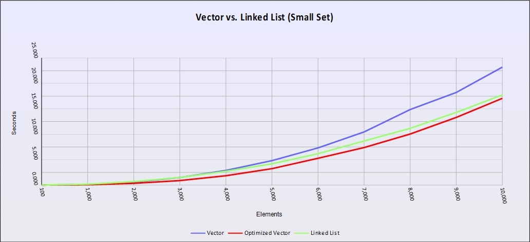
Figure 2 – Performance curves (load vs time) for std::list (green), std::vector (blue) and an optimized std::vector (red) using 4K buffers. A lower line means better performance.

 

The same code with a larger data size now performs very differently. Linked lists come into their own and not only erase the speed advantage of an array, they nearly erase the advantage of the optimized version.

That’s because blocks of our array no longer fit neatly into a cache line and the pre-fetcher is having to go back to main memory over and over again causing the same sort of cache misses we see in linked lists. Plus you have the overhead of inserting into an array which causes memory moves of large segments of memory.

The Take-aways:

• Always test your solutions because that’s the only true measure of performance. Our intuition is almost always wrong. In this case, complexity analysis was wrong about the outcome because complexity analysis fails to take into account the operational environment. Specifically, the effects of caching, the pre-fetcher, branch prediction and access patterns in memory.

• Treat operations involving -> as very expensive operations because they involve cache misses. That’s the primary reason that std::list failed so badly. std::vector used the same linear search that std::list used but because the pre-fetcher & branch predictor kept the cache full for us it performed much better.

• Know the standard algorithms. Knowing that lower_bound() is a binary search gives us a massive performance boost. It also simplified the algorithm and added some safety margin because looping through a vector using operator[] is somewhat dangerous in that it potentially allows us to run past the end of the vector without knowing it. Range-based for loops are a better choice.

• Understand the performance characteristics of the containers you’re using and know what specific implementations they use. std::multimap is typically built on a red-black tree while std::unordered_map is based on a hash table with closed addressing and buckets. Both are associative containers, but both have very different access patterns and performance characteristics.

• Don’t automatically assume that std::vector is always the fastest solution. That’s heresy today given how well it performs on cache-based hardware. With larger sized elements, though, it loses many of its advantages. And even though it’s not hard to roll a vector into an associative container, there are problems it does not handle well such as parsing (tries are better for that) or networks (directed graphs are better). Saying that all we need is a vector and a flat hash map with open addressing and local probing is a bit short-sighted.

• Don’t assume that the branch predictor, pre-fetcher or cache will make inefficient code run faster. In the vector implementation, it would be tempting to assume that reading vec.size() on each iteration instead of using count would be just as fast. In this case, that’s actually not true so test to be sure.

• Element size counts. Integers are small but if the items being accessed are large (structured data, say), linked lists erase a lot of that speed advantage that arrays have.

• Remember that complexity analysis is a measure of efficiency – not performance.